Python SDK

This article refers to Platform v3.0.0. The current Platform version is v3.4.0.

Overview

The barbara-sdk Python library lets you drive Barbara Panel from inside a Python program — typically a Jupyter notebook used for model training. You can list nodes, upload a trained model to the App Library, and deploy it to a node, all from a few function calls. This article walks through the SDK with a Titanic survival-prediction example.

barbara-sdk on PyPI

Features

• Upload trained models from Python or a Jupyter notebook to the Panel Library.
• Deploy models to edge nodes without leaving your training environment.
• Automate the full train → upload → deploy loop in scripts.
• Integrate edge AI development into the rest of your Python workflow.

Prerequisites

• Python 3.8 or newer.
• A Barbara platform account.
• Barbara API credentials:
  • username — your Panel account email.
  • password — your Panel account password.
  • client_id — provided by the Barbara support team.
  • client_secret — provided by the Barbara support team.

Barbara API credentials

API credentials are only available with an Enterprise license. Contact the Barbara support team if you need to upgrade.

Walkthrough — train and deploy a Titanic survival model

The example trains a small neural network that predicts whether a Titanic passenger survives, then uploads and deploys it from the notebook.

1. Install the library

pip install barbara-sdk

2. Download the example

titanic_notebook_example.zip

Download the Titanic example: titanic_notebook_example.zip.

Unzip the file. You will find:

File	Purpose
titanic_example.ipynb	Jupyter notebook with the full example.
titanic.csv	Passenger dataset.
credentials.json	Empty credentials file you need to fill in.

3. Fill in your credentials

Open credentials.json and replace the placeholders with the four API credentials.

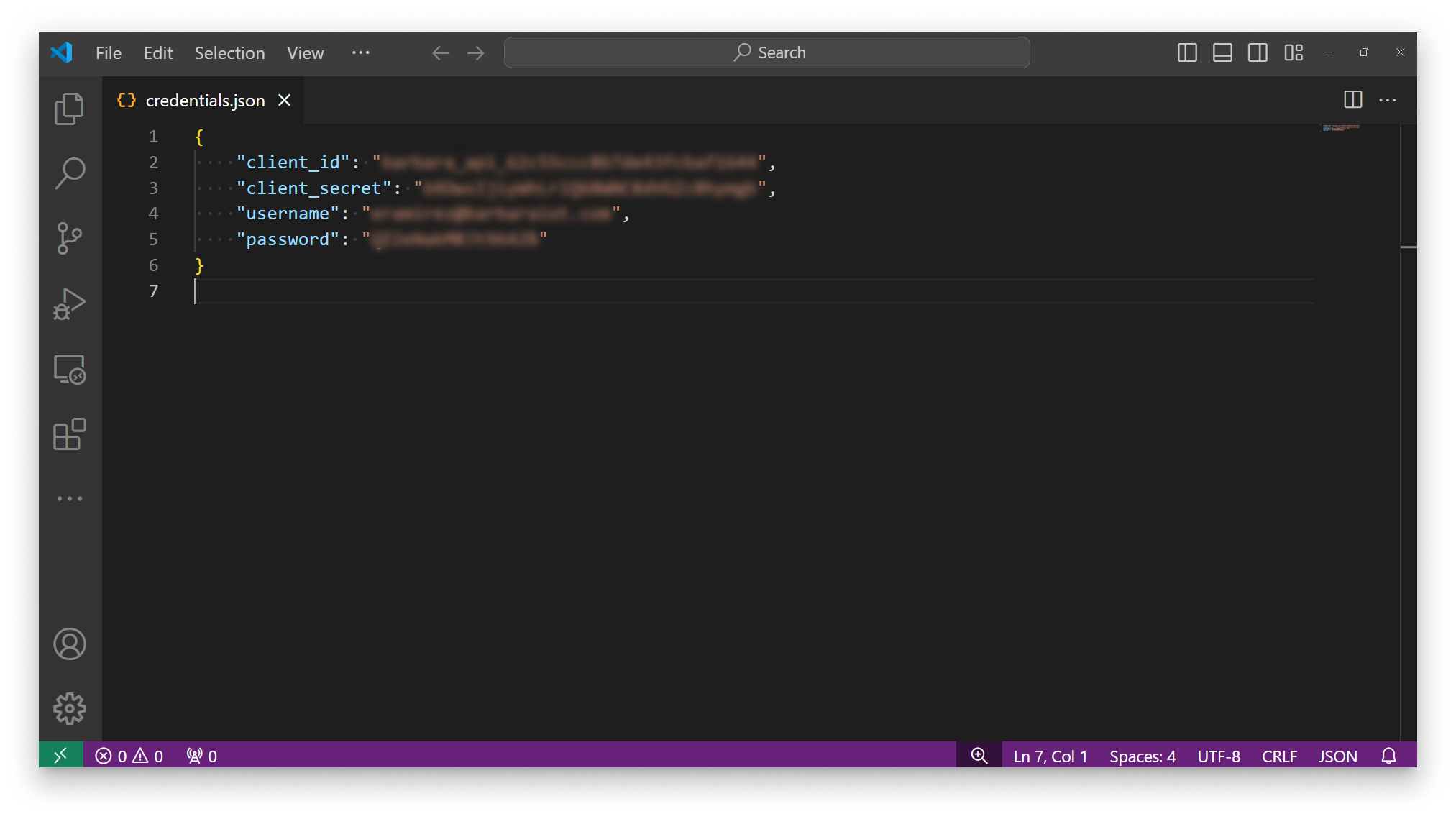
Fill in the credentials.json file

4. Open the notebook

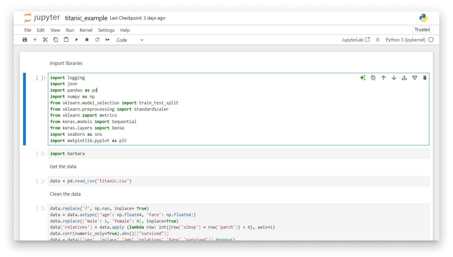
Titanic example in Jupyter notebook

Train the model

Imports

import json
import logging

import numpy as np
import pandas as pd
import seaborn as sns
import matplotlib.pyplot as plt
from sklearn import metrics
from sklearn.model_selection import train_test_split
from sklearn.preprocessing import StandardScaler
from keras.models import Sequential
from keras.layers import Dense

import barbara

Load the data

data = pd.read_csv('titanic.csv')

The CSV is read into a pandas DataFrame:

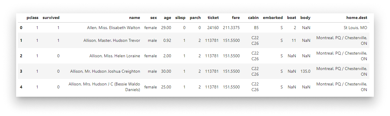
Raw Titanic data

Clean the data

Handle missing values, convert types, encode the sex column, and derive a relatives feature:

data.replace('?', np.nan, inplace=True)
data = data.astype({'age': np.float64, 'fare': np.float64})
data.replace({'male': 1, 'female': 0}, inplace=True)
data['relatives'] = data.apply(lambda row: int((row['sibsp'] + row['parch']) > 0), axis=1)
data = data[['sex', 'pclass', 'age', 'relatives', 'fare', 'survived']].dropna()

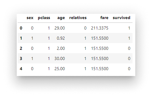
Cleaned Titanic data

Visualise

fig, axs = plt.subplots(ncols=3, figsize=(20, 3))
sns.violinplot(x="survived", y="age",  hue="sex", data=data, ax=axs[0])
sns.pointplot(x="pclass",   y="survived", hue="sex", data=data, ax=axs[1])
sns.violinplot(x="survived", y="fare", hue="sex", data=data, ax=axs[2])

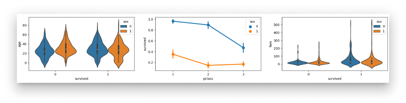
Survival plots by sex

Train / test split + standardisation

x_train, x_test, y_train, y_test = train_test_split(
    data[['sex', 'pclass', 'age', 'relatives', 'fare']],
    data.survived,
    test_size=0.2,
    random_state=0,
)

sc = StandardScaler()
X_train = sc.fit_transform(x_train)
X_test  = sc.transform(x_test)

Why standardise?

Standardisation puts every feature on the same scale (zero mean, unit standard deviation). Most ML algorithms converge faster and reach better accuracy when every input has a similar range.

Build and train the network

A tiny Keras Sequential model with two hidden layers of 5 ReLU neurons each, and a single sigmoid output:

model = Sequential()
model.add(Dense(5, kernel_initializer='uniform', activation='relu', input_dim=5))
model.add(Dense(5, kernel_initializer='uniform', activation='relu'))
model.add(Dense(1, kernel_initializer='uniform', activation='sigmoid'))
model.summary()

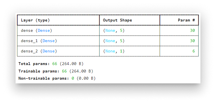
Keras model summary

Compile and train:

model.compile(optimizer="adam", loss="binary_crossentropy", metrics=["accuracy"])
model.fit(X_train, y_train, batch_size=32, epochs=50)

Test the model

y_pred = np.rint(model.predict(X_test).flatten())
print(metrics.accuracy_score(y_test, y_pred))

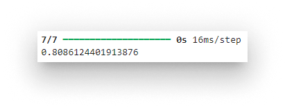
Test-set accuracy

Save the model

Export it in the layout the Barbara model wizard expects (<name>/<version>/):

model.export("titanic/1")

Deploy with the SDK

Authenticate

Load the credentials and instantiate the API client:

with open('./credentials.json') as f:
    cred = json.load(f)

logging.basicConfig(format='%(asctime)s %(levelname)s %(message)s', level=logging.INFO)

bbr = barbara.ApiClient(
    cred['client_id'],
    cred['client_secret'],
    cred['username'],
    cred['password'],
)

Upload the model

model_name = "Titanic"
bbr.models.upload("./titanic", model_name)

Inspect the Library:

bbr.models.list()

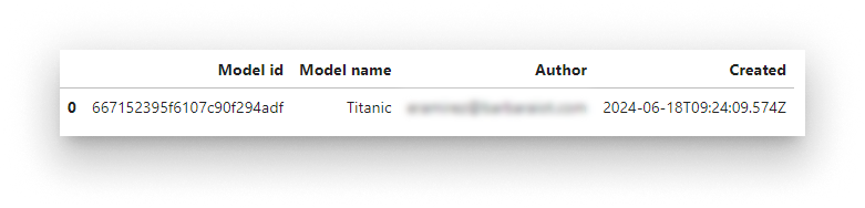
Models in the Library

List the versions of a specific model:

bbr.models.list_versions(model_name)

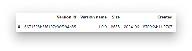
Versions of the Titanic model

Deploy to a node

List your nodes to pick the deployment target:

bbr.nodes.list()

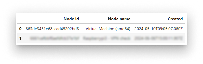
Edge nodes available to the account

Deploy:

node_name = "Virtual Machine (amd64)"
bbr.models.deploy(node_name, model_name)

Confirm the workload landed on the node:

bbr.workloads.list()

Workload list including the Titanic model

Operate the workload

Stop and start a workload by its ID:

workload_id = '666844535f6107c90fc2d6f6'
bbr.workloads.stop(workload_id)
bbr.workloads.start(workload_id)

Push a new version

Retrain locally, re-upload, and re-deploy in two calls:

bbr.models.upload("./titanic", model_name)
bbr.models.deploy(node_name, model_name)

Clean up

Remove the workload from the node:

bbr.workloads.remove(workload_id)

Remove the model from the Library:

bbr.models.delete(model_name)

Summary

The barbara-sdk lets you fold edge deployment into the rest of your Python workflow — from a Jupyter notebook you can train a model, upload it to the Library, deploy it to a node, and operate the resulting workload, all without context-switching to Panel. For the same operations from the UI, see the Models reference.